Matrix completion on graphs
Introduction
We try and implement a matrix recovery model with a simulated Netflix-like dataset. The aim is to model a simple recommender system on netflix. Given a fixed percentage of observations on the matrix users/movies, we want to recover all the values i.e the rating on each movie for each user.
The original problem lies on the hypothesis -often verified in practice- that a such users/movies matrix has a low rank.
Given a sparse set \(\Omega\) of observations \(M_{ij} : (i,j) \in \Omega \subseteq [ 1,\cdots,n] \times [1,\cdots,m]\), we want to find:
\[\min_{X \in \mathbb{R}^{m \times n}} ||X||_{\ast} s.t \mathcal{A}_{\Omega}(X)=\mathcal{A}_{\Omega}(M)\]Where \(\Vert X \Vert_{\ast}\) is defined as the classical nuclear norm.
By taking advantage of common caracteristics about users and movies, we can improve the original problem of matrix completation. The paper suggests the use of graph representation to handle this extra information. This notebook follows their experiments and shows the improvements over the original method to some extent.
A syntetic example of Netflix problem
# -*- coding: utf-8 -*-
import pandas as pd
from itertools import *
import collections
import numpy as np
import matplotlib.pyplot as plt
from cvxpy import *
import networkx as nx
%matplotlib inline
Let assume known information about users and movies, like age or sex, movies categories (War,Comedy, cartoons) or release date.
category = {'users' : {'sex' :['W','M'],
                     'age' :['<20','>50']},

            'movies' : {'genre':['Ca','Wa','Co'],
                      'release':['>2000','<1980']}
            }

tuplesU = list(product(*category['users'].values()))
tuplesM = list(product(*category['movies'].values()))

index = pd.MultiIndex.from_tuples(tuplesU,
                                    names=category['users'].keys())
columns = pd.MultiIndex.from_tuples(tuplesM,
                                  names=category['movies'].keys())

scores = [[3,2,4,3,1,3],[2,1,3,2,2,5],[2,5,2,4,1,2],[1,4,1,2,5,3]]
# buid table of scores by groups
scoresGroup = pd.DataFrame(index=index,columns=columns,data = scores)
print(scoresGroup)
genre      Ca          Wa          Co
release >2000 <1980 >2000 <1980 >2000 <1980
age sex
<20 W       3     2     4     3     1     3
    M       2     1     3     2     2     5
>50 W       2     5     2     4     1     2
    M       1     4     1     2     5     3
The table above gives rating for each category. For instance, a young boy is likely to like a recent war movie and dislike a comedy. This table of score is arbitrary and provides a toy example of a more real case.
Now we have to populate the users/movies matrix UM, according to the score matrix
- We define 10 to 12 individus in each group, namely the group of old men, old women, young boys and young girls
- For movies, there is 6 groups made up 6 to 8 movies.
nbU = np.random.randint(10,12,len(tuplesU))
nbM = np.random.randint(6,8,len(tuplesM))
The code below build the UM matrix, and shuffle rows and columns
# buid columns and index with hierachical level
def build_individus(name,nbInd):
    tuplesInd = list(product(*category[name].values()))
    u = []
    it=0
    for g,n in zip(tuplesInd,nbInd):
        u+=[g+ (i,) for i in range(it,it+n)]
        it +=n
    index =  pd.MultiIndex.from_tuples(u,
                                        names=list(category[name].keys())+[name])
    return index

# Mtrice Users/Movies creation
def build_matriceUM(nbU,nbM):
    A = pd.DataFrame(index=    build_individus('users',nbU),
                 columns = build_individus('movies',nbM))
    # fill the matrix according to scoresGroup
    for blockM,blockU in product(tuplesM,tuplesU):
        A.loc[blockU,blockM] = scoresGroup.ix[blockU].ix[blockM]
    # shuffle lign and columns
    A = A.sample(frac=1,axis=0)
    A = A.sample(frac=1,axis=1)
    return A

UM = build_matriceUM(nbU,nbM)
print(UM.head())
genre            Wa          Ca    Wa    Ca    Wa          Co    Ca    Wa  \
release       <1980 >2000 >2000 >2000 >2000 >2000 <1980 >2000 >2000 >2000
movies           20    13    1     15    5     18    21    31    0     19
age sex users
<20 M   13        2     3     2     3     2     3     2     2     2     3
>50 M   41        2     1     1     1     1     1     2     5     1     1
        39        2     1     1     1     1     1     2     5     1     1
        37        2     1     1     1     1     1     2     5     1     1
    W   27        4     2     2     2     2     2     4     1     2     2

genre          ...     Ca       Co       Ca             Co    Ca
release        ...  >2000    <1980    <1980          >2000 <1980
movies         ...     3  4     36 39    7  6  9  8     30    12
age sex users  ...
<20 M   13     ...      2  2     5  5     1  1  1  1     2     1
>50 M   41     ...      1  1     3  3     4  4  4  4     5     4
        39     ...      1  1     3  3     4  4  4  4     5     4
        37     ...      1  1     3  3     4  4  4  4     5     4
    W   27     ...      2  2     2  2     5  5  5  5     1     5

[5 rows x 40 columns]
The matrix of weights, for movies and users have to be created, according to group characteristics.
By instance, two young girls are linked in users matrix of weight by a 1.
A recent war movie and old one do not belong to the same group and a 0 will be add in the movies matrix weight
# Create matrix of weigths
def build_weight(index,group):
    Weight = pd.DataFrame(index = index,columns=index,data=0)
    for row,col in zip(group,group):
        Weight.loc[row,col]= 1 #nbOfCommonFeature
    return Weight

WeightU = build_weight(UM.index,tuplesU)
WeightM = build_weight(UM.columns,tuplesM)
print(WeightM.head())
genre                   Wa          Ca    Wa    Ca    Wa          Co    Ca  \
release              <1980 >2000 >2000 >2000 >2000 >2000 <1980 >2000 >2000
movies                  20    13    1     15    5     18    21    31    0
genre release movies
Wa    <1980   20         1     0     0     0     0     0     1     0     0
      >2000   13         0     1     0     1     0     1     0     0     0
Ca    >2000   1          0     0     1     0     1     0     0     0     1
Wa    >2000   15         0     1     0     1     0     1     0     0     0
Ca    >2000   5          0     0     1     0     1     0     0     0     1

genre                   Wa  ...     Ca       Co       Ca             Co    Ca
release              >2000  ...  >2000    <1980    <1980          >2000 <1980
movies                  19  ...     3  4     36 39    7  6  9  8     30    12
genre release movies        ...
Wa    <1980   20         0  ...      0  0     0  0     0  0  0  0     0     0
      >2000   13         1  ...      0  0     0  0     0  0  0  0     0     0
Ca    >2000   1          0  ...      1  1     0  0     0  0  0  0     0     0
Wa    >2000   15         1  ...      0  0     0  0     0  0  0  0     0     0
Ca    >2000   5          0  ...      1  1     0  0     0  0  0  0     0     0

[5 rows x 40 columns]
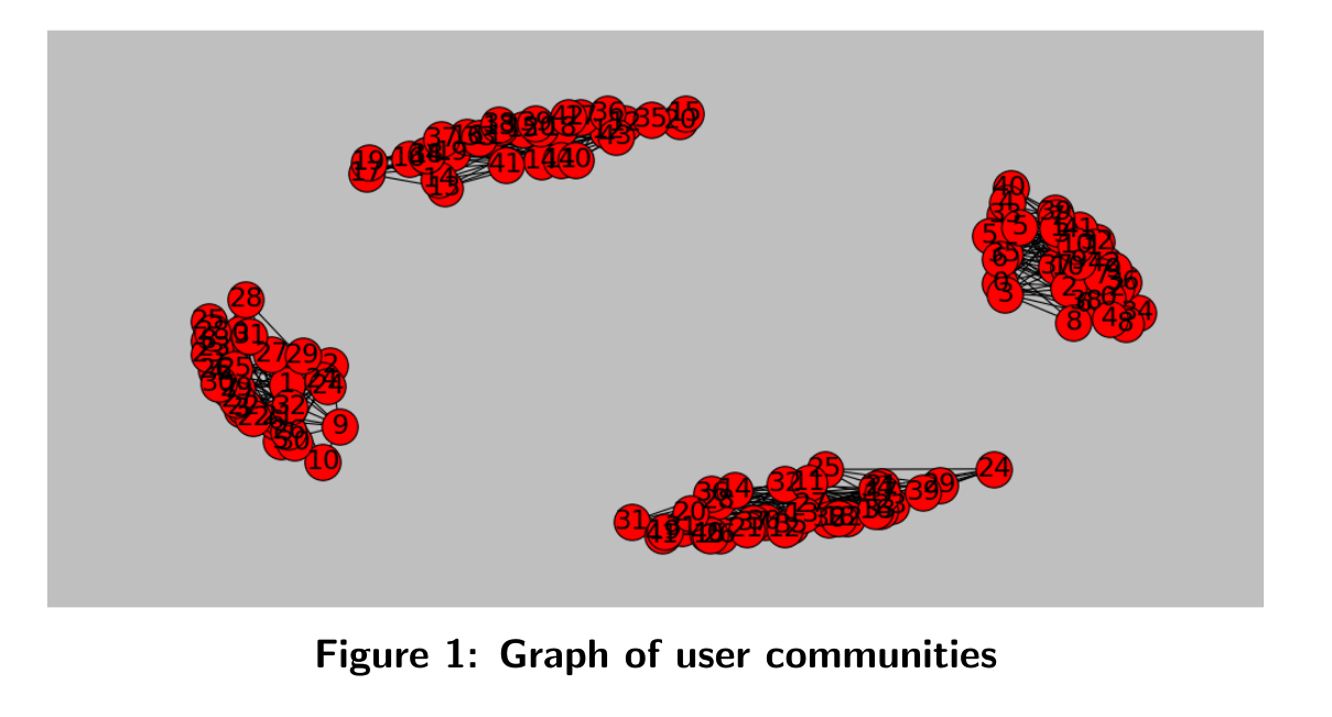
We can visualize graph of individus for instance with:
def plot_graph(Weight,level='users'):
    G=nx.Graph()
    # for all combinations between users, update weight graphs
    for tupleEdge in combinations(Weight.index.get_level_values(level),2):
        weight = Weight.xs(tupleEdge[0], level='users', axis=0).xs(tupleEdge[1], level=level, axis=1).values
        G.add_edge(*tupleEdge,weight=weight)
    #
    elarge=[(a,b) for (a,b,d) in G.edges(data=True) if d['weight'] ==1]
    pos=nx.spring_layout(G) # positions for all nodes
    # nodes
    nx.draw_networkx_nodes(G,pos,node_size=700)
    # edges
    nx.draw_networkx_edges(G,pos,edgelist=elarge,
                        width=1)
    nx.draw_networkx_labels(G,pos,font_size=20,font_family='sans-serif')
    plt.axis('off')
    plt.show() # display
plot_graph(WeightU,'users')
Let assume that we have partial measurements of \(UM\). Some users have scored some movies, but UM entries has a lot of empty spaces. Let us observe 5% for the next examples of the \(UM\) matrix. The goal is now to rebuild it.
def mask(u, v, proportion = 0.3):
    mat_mask = np.random.binomial(1, proportion, size =  (u, v))
    print("We observe {} per cent of the entries of a {}*{} matrix".format(100 * mat_mask.mean(),u, v))
    return mat_mask

mat_mask = mask(*UM.shape,proportion=0.05)
UM_mask = mat_mask*UM
We observe 5.11904761905 per cent of the entries of a 42*40 matrix
Let us recall the original problem
The matrix of weights are not used here, so we want to find :
\[\min_{X \in \mathbb{R}^{m \times n}} ||X||_{\ast} s.t \mathcal{A}_{\Omega}(X)=\mathcal{A}_{\Omega}(M)\]The library CVXPY provide user-friendly tools to define this problem
X = Variable(*UM.shape)
obj = Minimize(norm(X, 'nuc') )  # norm nuclear: hypotesis of low rank
constraints = [mul_elemwise(mat_mask, X) == mul_elemwise(mat_mask, np.array(UM))]
prob = Problem(obj, constraints)
prob.solve(solver=SCS)
UM_rebuild = pd.DataFrame(index = UM.index,columns=UM.columns,data=X.value)
def rmse(A,B):
    rmse = ((A-B).values**2).mean()
    print("RMSE: %.2f" %rmse)
    return rmse
The RMSE of the recovered solution can be find:
rmse(UM,UM_rebuild)
RMSE: 6.68
With the information of similar rating over groups:
Now, by putting aside low rank hypothesis, the intuition is to force two different vectors of users noted \(x_{i}\) and \(x_{i'}\) to be closed when their respective link \(w_{ii'}^{u}\) are not zero. \(w_{ii'}^{u}\) is the entries of the matrix of weight for users \(W^{c}\). Namely, we want to find \(X \in \mathbb{R}^{m*n}\) minimizing ;
\[\sum \limits_{i,i'} w_{ii'}^{u}\Vert x_{i}-x_{i'}\Vert_{2}^{2} = tr(XL_{u}X^t) = \Vert X \Vert^2_{\mathcal{D},u}\]We then define positive semidefinite matrix \(L^{u}\) defined as \(D^{u}-W^{u}\) where is defined such that : \((D^{u})_{ij} = diag(\sum_{j=1}^{m} W_{ij}^{u})\)
The same idea is applied for movies vectors.
So, the problem of matrix completion can be formulated as follows :
\[\min_{X} \frac{\gamma_u}{2}||X||^2_{\mathcal{D},u}+\frac{\gamma_m}{2}||X||^2_{\mathcal{D},m}\]def build_L(Weight):
D = np.diag(Weight.sum(axis=0))
L = (D-Weight).values
return L
LM = build_L(WeightM)
LU = build_L(WeightU)
It is not that easy to find a procedure minimizing \({\Vert X\Vert}^{2}_{\mathcal{D},u}\).
We have expressed \(X\) in other basis. In order to take benefit from the cvxpy toolbox. Indeed, we can use \(tr(XX^{t})=\Vert X\Vert ^2_{\mathcal{F}}\), which is the square of the Frobenius norm.
More precisions may be found in our report.
def change_basis(L):
    V,P = np.linalg.eigh(L) # diagonalise
    V1 = np.diag(np.sqrt(np.abs(V)))
    P1 = np.dot(P,V1)
    return P1
PM1 = change_basis(LM)
PU1 = change_basis(LU)
X = Variable(*UM.shape)
obj = Minimize(norm(X*PM1, 'fro') + norm((PU1.T)*X, 'fro')) # norm frobenius: information from graphs
constraints = [mul_elemwise(mat_mask, X) == mul_elemwise(mat_mask, np.array(UM))]
prob = Problem(obj, constraints)
prob.solve(solver=SCS)

UM_rebuild = pd.DataFrame(index = UM.index,columns=UM.columns,data=X.value)
rmse(UM,UM_rebuild)
RMSE: 1.04
The rmse is here better than the first case.
Comparision of those methods, under several scenarios
To assess the improvement from graphs information, a lot of cases have been simulated. We wanted to compare the performances in term of RMSE for the matrix completion problem with:
- Nuclear norm, based on low rank hypothesis
- Graph information
- The combination of both
Under several scenarios:
- With noise in the matrix of weight. Some 1 have been added, creating a wrong link, or some 0 have replaced 1, removing a correct link.
- With different percentages of \(UM\)’s observation.
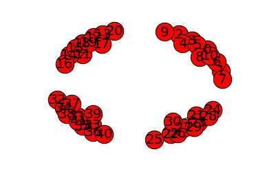
To add noise, we can use a XOR provided by numpy to flip the bits of the matrix of weight. We delete some links inside the communities or create ones between them:
WeightU_noise =  np.logical_xor(WeightU,mask(*WeightU.shape,proportion=0.1))
plot_graph(WeightU_noise,'users')
We observe 10.0340136054 per cent of the entries of a 42*42 matrix
# optimization problem inside a function
def rebuild(nuc,fro,PM1,PU1,mat_mask):
    X = Variable(*UM.shape)
    obj = Minimize(nuc*norm(X, 'nuc') +  # norm nuclear: hypotesis of low rank
                   fro*(norm(X*PM1, 'fro') + norm((PU1.T)*X, 'fro'))) # norm frobenius: information from graphs
    constraints = [mul_elemwise(mat_mask, X) == mul_elemwise(mat_mask, np.array(UM))]
    prob = Problem(obj, constraints)
    prob.solve(solver=SCS)
    UM_rebuild = pd.DataFrame(index = UM.index,columns=UM.columns,data=X.value)
    return UM_rebuild
The dataframe containing results is now created
dic_result={'noise':range(0,40,10),
            'nuc':[0,1],
            'fro':[0,1]}

result = pd.DataFrame(index=pd.MultiIndex.from_product(dic_result.values(),
                                                       names=dic_result.keys()),
        columns=range(0,80,10))
result = result.ix[~((result.index.get_level_values('nuc')==0) & (result.index.get_level_values('fro')==0))]
print(result.head())
                0    10   20   30   40   50   60   70
noise fro nuc
0     0   1    NaN  NaN  NaN  NaN  NaN  NaN  NaN  NaN
      1   0    NaN  NaN  NaN  NaN  NaN  NaN  NaN  NaN
          1    NaN  NaN  NaN  NaN  NaN  NaN  NaN  NaN
10    0   1    NaN  NaN  NaN  NaN  NaN  NaN  NaN  NaN
      1   0    NaN  NaN  NaN  NaN  NaN  NaN  NaN  NaN
The loops to fill it:
for observation in result.columns:
    proportion = observation/100.
    mat_mask = mask(*UM.shape,proportion=proportion)
    for noise,fro,nuc in product(*result.index.levels):
        if ~((nuc==0) & (fro==0)):
#            print(noise,fro,nuc)
            WeightM_noise = np.logical_xor(WeightM,mask(*WeightM.shape,proportion=noise/100.))
            WeightU_noise =  np.logical_xor(WeightU,mask(*WeightU.shape,proportion=noise/100.))
            LU_noise = build_L(WeightU_noise)
            LM_noise = build_L(WeightM_noise)
            UM_rebuild =  rebuild(nuc,fro,
                                  change_basis(LM_noise),
                                  change_basis(LU_noise),mat_mask)
            r = rmse(UM_rebuild,UM)
            result.loc[(noise,fro,nuc),observation] = r
We observe 0.0 per cent of the entries of a 42*40 matrix
We observe 0.0 per cent of the entries of a 40*40 matrix
We observe 0.0 per cent of the entries of a 42*42 matrix
RMSE: 8.57
We observe 0.0 per cent of the entries of a 40*40 matrix
We observe 0.0 per cent of the entries of a 42*42 matrix
RMSE: 8.57
We observe 0.0 per cent of the entries of a 40*40 matrix
We observe 0.0 per cent of the entries of a 42*42 matrix
RMSE: 8.57
We observe 10.5625 per cent of the entries of a 40*40 matrix
We observe 9.92063492063 per cent of the entries of a 42*42 matrix

......

We observe 31.625 per cent of the entries of a 40*40 matrix
We observe 29.8185941043 per cent of the entries of a 42*42 matrix
RMSE: 0.00
We observe 30.25 per cent of the entries of a 40*40 matrix
We observe 31.9160997732 per cent of the entries of a 42*42 matrix
RMSE: 0.47
We observe 30.6875 per cent of the entries of a 40*40 matrix
We observe 29.9319727891 per cent of the entries of a 42*42 matrix
RMSE: 0.08
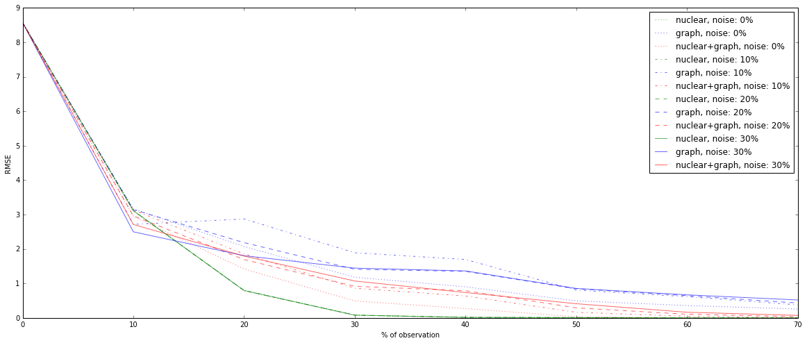
It yields to the next graphs, showing the effect of noise, for different percentages of observation:
fig = plt.figure(figsize=(20,8))
ax = fig.add_subplot(111)
color_dic = {(0,1):'b',(1,1):'r',(1,0):'g'}
style_dic = {k:v for k,v in zip(dic_result['noise'],[':','-.','--','-'])}
result.loc[(slice(None),1,1),:]
for noise,fro,nuc in  product(*result.index.levels):
    if ~((nuc==0) & (fro==0)):
        label = nuc*'nuclear'+ nuc*fro*'+'+ fro*'graph' +', noise: '+ str(noise)+ '%'
        result.loc[(noise,fro,nuc),:].T.plot(color = color_dic[(nuc,fro)],
                                            style=style_dic[noise],
                                            label=label,
                                            alpha = 0.6)
ax.legend()
ax.set_xlabel('% of observation')
ax.set_ylabel('RMSE')
<matplotlib.text.Text at 0x29143898>
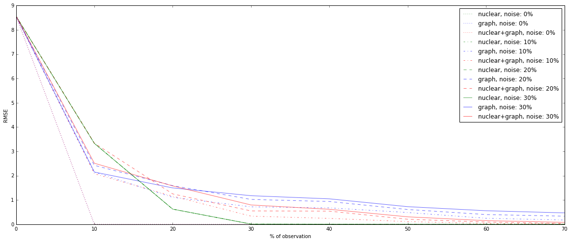
As we can show, information of communities is very strong, and outperforms the original problem if there is no noise. In case of noise for the matrix of weights, 30% of wrong links for instance, the first problem based on nuclear norm minimization gets better result from more than 10% of observations.
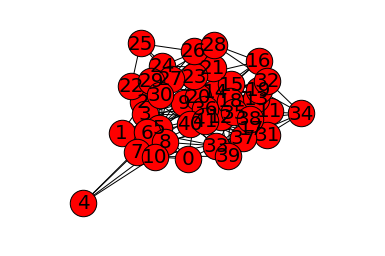
To be more realistic, the matrix of weight have been made sparser. The half of links is removed:
WeightU = WeightU*mask(*WeightU.shape,proportion = 0.5)
WeightM = WeightM*mask(*WeightM.shape,proportion = 0.5)
We observe 52.2675736961 per cent of the entries of a 42*42 matrix
We observe 49.125 per cent of the entries of a 40*40 matrix
The same fillling is done:
for observation in result.columns:
    proportion = observation/100.
    mat_mask = mask(*UM.shape,proportion=proportion)
    for noise,fro,nuc in product(*result.index.levels):
        if ~((nuc==0) & (fro==0)):
#            print(noise,fro,nuc)
            WeightM_noise = np.logical_xor(WeightM,mask(*WeightM.shape,proportion=noise/100.))
            WeightU_noise =  np.logical_xor(WeightU,mask(*WeightU.shape,proportion=noise/100.))
            LU_noise = build_L(WeightU_noise)
            LM_noise = build_L(WeightM_noise)
            UM_rebuild =  rebuild(nuc,fro,
                                  change_basis(LM_noise),
                                  change_basis(LU_noise),mat_mask)
            r = rmse(UM_rebuild,UM)
            result.loc[(noise,fro,nuc),observation] = r
We observe 0.0 per cent of the entries of a 42*40 matrix
We observe 0.0 per cent of the entries of a 40*40 matrix
We observe 0.0 per cent of the entries of a 42*42 matrix
RMSE: 8.57
We observe 0.0 per cent of the entries of a 40*40 matrix
We observe 0.0 per cent of the entries of a 42*42 matrix
RMSE: 8.57
We observe 0.0 per cent of the entries of a 40*40 matrix
We observe 0.0 per cent of the entries of a 42*42 matrix
RMSE: 8.57

.....

We observe 20.1875 per cent of the entries of a 40*40 matrix
We observe 21.1451247166 per cent of the entries of a 42*42 matrix
RMSE: 0.04
We observe 30.5 per cent of the entries of a 40*40 matrix
We observe 30.3854875283 per cent of the entries of a 42*42 matrix
RMSE: 0.00
We observe 30.5625 per cent of the entries of a 40*40 matrix
We observe 31.4058956916 per cent of the entries of a 42*42 matrix
RMSE: 0.52
We observe 28.3125 per cent of the entries of a 40*40 matrix
We observe 30.1020408163 per cent of the entries of a 42*42 matrix
RMSE: 0.07
fig = plt.figure(figsize=(20,8))
ax = fig.add_subplot(111)
color_dic = {(0,1):'b',(1,1):'r',(1,0):'g'}
style_dic = {k:v for k,v in zip(dic_result['noise'],[':','-.','--','-'])}
result.loc[(slice(None),1,1),:]
for noise,fro,nuc in  product(*result.index.levels):
    if ~((nuc==0) & (fro==0)):
        label = nuc*'nuclear'+ nuc*fro*'+'+ fro*'graph' +', noise: '+ str(noise)+ '%'
        result.loc[(noise,fro,nuc),:].T.plot(color = color_dic[(nuc,fro)],
                                            style=style_dic[noise],
                                            label=label,
                                            alpha = 0.6)
ax.legend()
ax.set_xlabel('% of observation')
ax.set_ylabel('RMSE')
<matplotlib.text.Text at 0x2b6cf1d0>
With partial information of communities membership, the results are worse. Basically, for 10% of observation, graph-based resolution is still better, but after, nuclear norm based optimization becomes more accurate.